Γενικά
In the following guide you will find references and details regarding both the proper functioning of the program, the implementation of regulations and the appearance of the results in SCADA Pro. You will also find improvements and corrections that offer greater ease of use and accurate results.
Development & Improvements
The main objective of ACE-Hellas is the continuous development, offering its customers solutions functional and effective. For this reason, the company’s development department takes care to continually update the programs according to the new norms, new market needs and of course the user requirements.
Clarifications
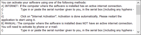
1. 1. How to activate the program into a computer, how to deactivate and back on, to the same or to another?
After buying the program, the user recieves the serial number.
The serial number has the following characteristics:
- Consists of 16 digits, numbers and characters, separated by four dashes
- It is unique and includes all the purchased Modules.
- Any subsequent purchase of one or more of the same version Module added to the same serial, without requiring any changes by the user.
- Upgrading to the next version requires a new Serial Number.
The program can be installed on as many computers as you like, but can only be active in one.
You can enable or disable the program, easily, as many times as you like, in the same or another computer.
To activate the program:
The first time you open the application, inside the environment of the program appears the window for activation.
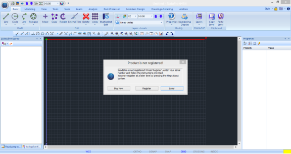
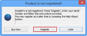
Press Register to open the dialog:
NOTE: The same window opens by clicking the button with the padlock in the program window, above on the right.
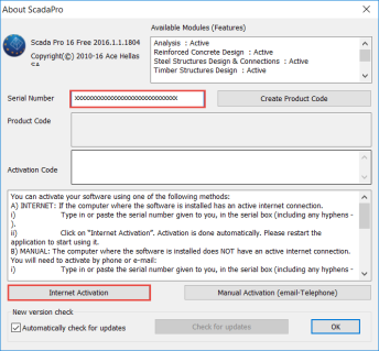
– Enter the Serial Number,
– Press Internet activation and
– The program is activated automatically.
NOTE: If you do not have Internet connection, follow the activation instructions written on it.
When the program is activated, the field with the serial number deactivated and the command where prior was written Internet Activation now writes Internet Deactivation.
To deactivate the program:
Open the program and press the command with padlock

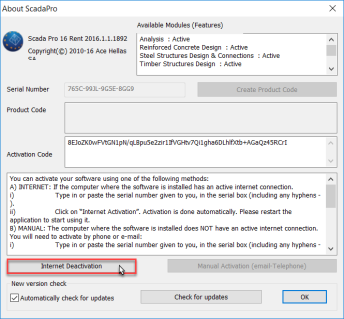
– Press Internet Deactivation and
– The program is deactivated automatically.
Now you can activate the software on another computer.
2. How to name the files of SCADA;
Prerequisite to make the program commands work, is to give a name to the file.
The file name must be composed of a maximum of 8 characters and / or numbers without spaces and without the use of special characters (/, -, _) (ex FILE1). The program automatically creates a folder that stores all the details of your project. The “position” of the file, ie the point where this file will be created, should be located on the hard disk. We propose to create a folder in C (ex PROJECTS), where all projects of SCADA will be located (ex C: \ PROJECTS \ FILE1)
ATTENTION: The entire path should be in Latin characters and / or numbers without spaces and without the use of special characters.
3. What files must erase to delete analysis or dimensioning scenarios;
The program automatically creates a folder with the given name that contains subfolders, ready to welcome all the details of the project. Specifically, in each subfolder are:
scanal:analysis files
scades_c:design files of concrete structural elements
scades_Sid:design files of steel structural elements
scades_Synd:design files of the steel connections
scainp:input files of the linear structural elements (i.e. beams, columns)
and the slabs
scapush:pushover analysis files
scatmp:temporary files
tmp:temporary files
project.inf:data base information
So if you want to delete the analysis scenarios, is sufficient you delete the folder scanal and respectively for dimensioning scenarios the corresponding scades folder.
ATTENTION: Erasing those files imply the deletion of the default analysis scenarios and dimensioning respectively. Therefore, in the corresponding windows Scenario>New there will be no longer predefined scenarios. Means that the user should create from the beginning the list of the scenarios, specifying all parameters (ex the units in Load Cases).
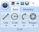
Modeling
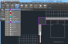
4. How to use a dwg/dxf file as an auxiliary file;
The introduction of an auxiliary dwg / dxf file can be used in different ways.
- Simple introduction, works as a platform, offering,
– either span points on the drawing lines, for the manual mode,
– or contours, for the semiautomatic way of inserting elements with manual selection.
- By using the dwg / dxf command, providing a fully automated tool that enables the reproduction of a single floor plan to selected floors and the automatic creation of the model. The use of this command sets certain requirements on the design of the dwg / dxf file, in order to identify the sections and create a static model of the project.
5. How should be made the dwg / dxf file to be used as an auxiliary;
For using a dwg/dxf file as un auxiliary file should be designed so that:
–  Each floor plan that will be used as an auxiliary file should reside on a separate file that does not include other projects beyond the current floor plan with all the design entities.
– Lines or/and polylines defining the columns, or the beams and the cantilevers, should belong to three different separate layers.
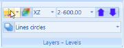
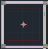
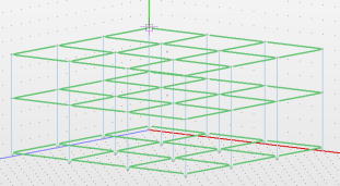
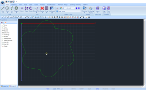
– The auxiliary file is inserted in the SCADA environment in active XZ level, matching the origin to the upper left point of the project ![]() . When entering more auxiliary designs in elevation, take care of the insertion point as to obtain the correct height continuity of floors
. When entering more auxiliary designs in elevation, take care of the insertion point as to obtain the correct height continuity of floors
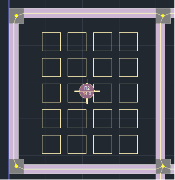
Floor Plan 1 (SCADA)
Floor Plan 2 (SCADA)
Summarizing all the above, we conclude that: the dwg / dxf file to use for the automatic recognition should include a single floor plan.
In cases of projects without typical floor, or with more typical floors, or with completely different floorplans in height there is a need for introducing more auxiliary files.
SCADA allows the user to introduce as many dwg / dxf files wishes (provided that each one comprise a floor plan only). These are saved in the project file and can be used to generate the static model, combining the fully automatic mode, the semi-automatic and manual.
6. Differences between Automatic and Manual process of the model creation of dwg / dxf
Let’s see in detail how operates these the two processes in order to identify the differences and understand why the selection “Auto Insert connecting beams” is disabled when the project file has been created,
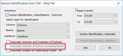
while happens the opposite in the initial automatic process.
Automatic Process
In this process, which can be selected from the start of the program, we can only import a dwg / dxf which always goes to the 0 level.
So, since we define the projects levels:
in the dialog box of automatic recognition:
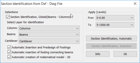
declare as usual the layers and automatically comes the overall recognition of a model.
There are two points that needs attention:
α) The functional of the automatic process is that first identifies (creates) physical entities as the columns and beams to the level introduced the dwg / dxf (0 level) and then copies them to the levels specified in the section “Apply.” 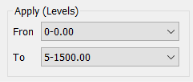
So, the elements will be, on the insertion level and the “Apply” levels. Of course, the same reasoning followed the manual process that will see below.
β) Activating ![]() , converts the identified beams to the dwg inserting level (level 0) in connecting beams with the same dimensions. Deactivating this choice does not recognize any beams at level 0.
, converts the identified beams to the dwg inserting level (level 0) in connecting beams with the same dimensions. Deactivating this choice does not recognize any beams at level 0.
Manual Process
Before describing the steps, we need to follow the manual process must be emphasized that this gives us the flexibility to introduce different dwg / dxf per level, that’s why this mode is a little different. This means working by levels.
The first step is to start a new file, and create the levels.
Then, import the dwg / dxf file in the first level of the structure (the first level above the foundation level) and if the floor is typical choose the command ” Sections Identification “-> “Columns” and recognize the items (Columns, Beams) in the import level and those defined in “Apply” (Attention! This application concerns only levels above ground).
If we do not have typical floor, repeat the above process to those levels above ground we have introduced different dwg / dxf.
Finally we go in the foundation level and introduce the dwg / dxf file containing the data foundation or at the floor plan that contains the columns that lead to the foundation and the beams on which positions we want to create connecting beams.
Then select the command “ Elements Creation from DXF/DWG” -> “Foundation Beams“
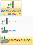
which recognize columns and connections beams.
In the dialog box that appears:
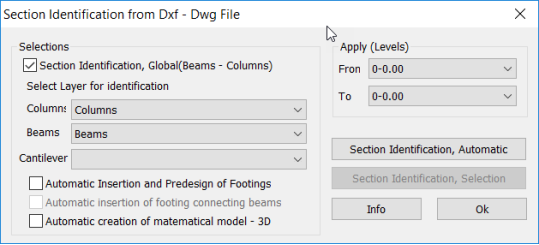
select “ Section Identification, Global “, we define as usual the layers and choose “Apply” to level 0 (even From and To) or the foundation levels (From – To) if there are more than one.
NOTES for the manual process:
- Because there is a separate command for the recognition of the foundation elements, the “Auto Insert connecting beams” is meaningless and is disabled.
- Because the manual element identification process takes place in two steps (foundation and superstructure) is meaningless the “Automatic Creation of Mathematical Model – 3D”, that’s why is inactive by default.
- Because of the gradual process of the manual method, also “Automatic Insertion and Predesign of Footings” is unable, because the loads are not defined for the predesigning.
7. How to create indirect supports (beam on beam)
NOTE: The “Beam on Beam” command concerns only the physical sections of beams, meaning that is used before the creation of the mathematical model.
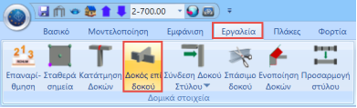
This command is used to define indirect support between the beams.
Select the command and then left click on the first beam and then on the second beam.
The individual cases are analyzed in the following examples:
- EXAMPLE 1
Aim: To create an indirect support between beam 1 and beam 2.
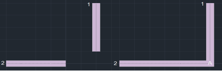
Select the command and then the beams 1 and 2. After the creation of the mathematical model, the node of the indirect support will be generated, in position “A”.
- EXAMPLE 2
Aim: The definition of a T-shaped indirect support of two beams.
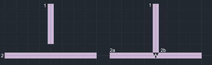
Draw the beam 1 and stop just before drawing beam 2. Select the command and click sequentially on the two beams. The order does not matter. Then, after the mathematical model creation, in position A (see Figure) the node of the indirect support will be created and beam 2 will break in two parts 2a and 2b.
- EXAMPLE 3
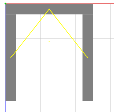
Aim: The definition of a “+” shaped indirect support between two beams.
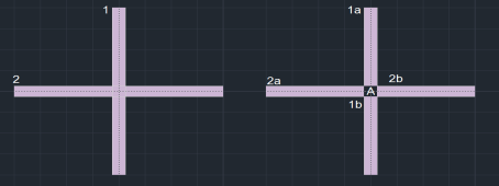
Draw beams 1 and 2. Select the command and click on the two beams sequentially. The order does not matter. Then, after the mathematical model creation, in position A (Figure) the node of indirect support will be created and the beams 1 and 2 will break in two parts each (1a, 1b, 2a, 2b).
- EXAMPLE 4
Aim: The definition of a multiple indirect support between more beams.
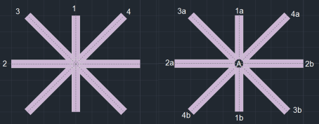
First create the node of indirect support between beams 1 and 2 (cross). Then, insert beam 3 and beam 4 and select again “Beam on Beam” command. Click sequentially on the two beams.
NOTES for the Automatic Identification process of the dwg / dxf file:
- Because in the automatic recognition process the option “Automatic Creation of Mathematical Model – 3D” is enabled, in those cases where are indirect supports, you have to intervene manually, initially deleting the mathematical model of the beams of indirect supports, then using the same command and calculating the mathematical model again.
- During designing of indirect support in the dwg/dxf file, draw the entire beams, and not the parts of these, to make them easier to edit in SCADA.
8. How to create Planted Columns
NOTE: To insert a planted column use the same command used for the regular columns.
ATTENTION: Planted column should “stand” on a beam (there is no planted column on slab).
LOWER LEVEL (base of planted column)
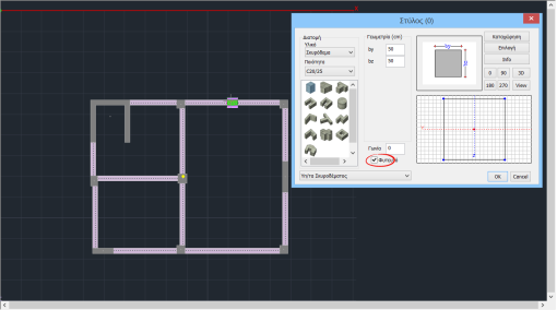
Activate the level where planted column “stands” (base of planted column), select the command “Modeling>Column” and in the dialog box, define the characteristics of the column and activate “Planted”.
Using the snaps, iindicate by left-click the insertion point of the “planted” on the beam.
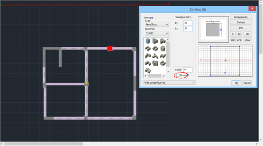
UPPER LEVEL (top of planted column)
Repeat the process, activating now the top level, and insert the section of the top of the “planted” column on the beam, but with “Planted” indication now Inactive.
Finally, choose the mathematical model calculation and complete modeling of “planted” column.
9. How to copy one or more physical elements from one level to another
NOTE: The commands for copying, either individual elements ![]() , or the entire level
, or the entire level ![]() concern only the physical sections! Meaning that are used before the creation of the mathematical model.
concern only the physical sections! Meaning that are used before the creation of the mathematical model.
ATTENTION: The elements with mathematical model does not obey these commands, and you should use the respective “Create Clone” command.
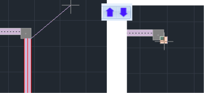
Use left mouse button to indicate the characteristic point (end of a line, top of a column, end of a beam, etc) which defines “from here”, move using the arrow to the new level and choose there the next characteristic point that defines “to there”.
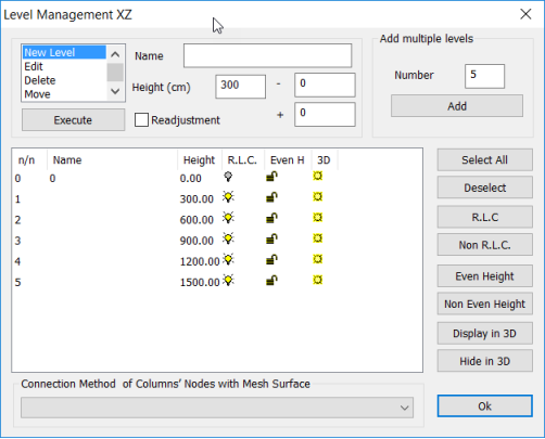
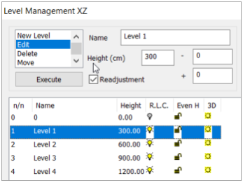
10. How to manage the levels
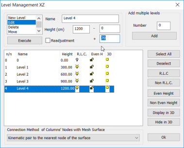
“Level Management” command 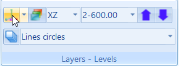 allows the creation and editing of levels.
NOTES:
– The floor plan level is on the global X-Z and Y is the perpendicular to this axis.
– Level 0 for SCADA the foundation level.
– In SCADA never define negative elevations.
– For SCADA, 0 is the level where the foundation “begins” (the base of the foundation element)
– Consequently, the altitude of level 1 will include also the height of the foundation. If for example the foundation is 1m height and the floor is 3m, the levels 1 elevation, will be 4m (400cm).
– When foundation is situated in different heights, you could
even define level 1 as the second foundation level (switch off R.L.C. (Rigid Link Constrain)),
or define an “irregularity” in the existing level 0 (see question How to define an irregularity level?), using “Move with Attachments” command.
- To define levels,
select “New level”, type “Name” and “Height” and press Execute, repeating for all levels of the structure,
or enter the number of floors in the field “Add multiple Levels”, and after setting a Height, select Add. Just a single step for creating all building levels!
Fields – and +, complemented where there are irregularities or inclination or existence of vertical surface elements, so that the elements comprising belong at this level (for the distribution of the masses) and displayed at this level.*
* For example, the 2nd level height 700 cm contains un irregularity on 600 cm. In the field “-“ type 150 (cm). Thus, when activates the 2nd level, apart from the entities belonging to the level 2, would appear also all those elements located to 150 cm below it.
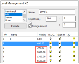
- To modify an existing level,
select “Edit” and a level from the list to turn blue, type a new “Name” or a new “Height” and “Execute”.
Activating “Readjustment” before “Execute”, modifies the altitudes of the highest floors according to the modification is the lower level *
* If, for example, modify the first level with an initial altitude of 300 cm, setting a new altitude 400 activating “Readjustment”, all the levels above 1 will be adjusted accordingly. Otherwise modified only the altitude of the selected level.
To delete a level and all items belonging to it,
Choose the level, the 1st “Delete” and “Execute”. This deletion removes the level and all items belonging to it.
To delete only the level and not the elements belonging to this,
Choose the level, the 2nd “Delete” and “Execute”. This deletion removes only the level and not the items belonging to it.
Using “Move” command, you can move a level from one location in the list, to the next position. Choose the level to move, select “Move” from the work menu and then select the “Execute” button. The level moves one position below. This command is useful in cases where you want to insert a level between other levels and the initial creation of this level was not in the right position, but at the end of the list.
11. How to define an irregularity level
The command used to transfer objects from one level, creating irregularities, is “Move with Attachments“.
Firstly, select the command and then the objects to be moved by using the “window or polygon” option. The objects inside the window are moved, while the objects that are intersected by the window are stretched. During moving and stretching the mathematical model of the selected elements is also included.
- Starting with “Level Management ΧΖ”, edit for example Level 4, stating the irregularity (+ 70), and “Execute”.
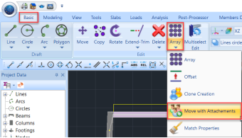
- Select: “Basic”-”Array”–“Move with Attachment”.
- Use Window selection, to select the nodes that will change altitude and right click.
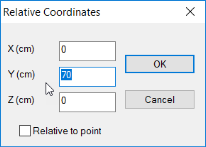
- Left click on a node and select
 .
. - Type the irregularity height in Υ (70 cm) and OK.
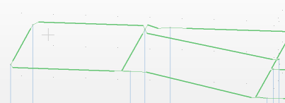
- Next step is to modify the rigid offsets authority or end (depending on the time they are placed on the floor plan) of the sloping beams, that they leveled.
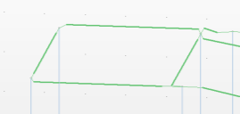
In the beam located between slab irregularities, give Zeta section characteristics.
Select the beam and press More “… “ in Properties:
NOTE: About the Rigid Link Constrain of the level comprising irregularities, you could either release all nodes belonging in the irregularity from the diaphragm node, or not to include it, deleting the diaphragm node of this level, of course assuming an unfavorable situation.
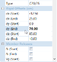
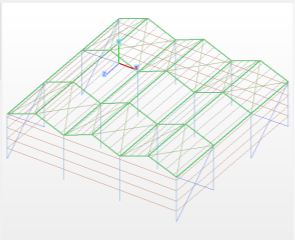
12. How to create a sloping roof
The process for creating the inclined roof is similar to create an irregularity.
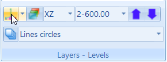 Start again with “Level Management ΧΖ”, and edit the level (2 for example), stating au irregularity (+ 70, for example).
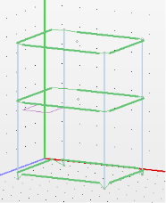
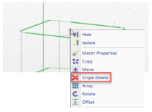
- Delete the diaphragm node of the level, using right–click> Delete one (if there are more slabs in the same level, then you release the nodes of the inclined plate from the diaphragm)
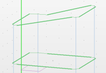
- Create the irregularity using Move with Attachment and the relative coordinates (see. How to define an irregularity level)
NOTE:
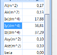
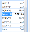
If you want to simulate the diaphragm function on the roof slab, you can multiply the moment of inertia Iy of the parametrical beams, by a factor (50-100).
13. Calculation and deletion of the mathematical model
The creation of the mathematical model is required when the model is created using the physical sections and/or mesh.
The calculation of the mathematical model means the attribution of the inertial properties, the connection between the model elements and the possibility of the 3dimensional visualization and rendering. The calculation of the mathematical model can be done repeatedly. You can also, delete it all or part of it and recalculate it.
The need for deletion and recalculation occurs frequently, either to use the program commands that work only in the physical model (beam on beam, beam break or consolidation, etc.), or to make copies and transfers, or for other reasons.
The deletion could be selectively, by deleting a member or a node, using Delete command, or globally for the entire project or only from the current level.
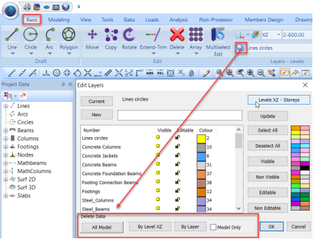
The command for total deletion is in “Edit Layer” window, at the bottom:
![]()
|
|
This command is used for erasing the mathematical model of the project. |
|
|
Erase the elements belonging to the selected layers from the current ΧΖ level. Firstly, select one or more layers, then deactivate “Model Only” checkbox and finally click “By Level ΧΖ”. |
|
|
Erase the mathematical model of the elements belonging to the selected layers from the current ΧΖ level. Firstly, select one or more layers, then activate “Model Only” checkbox and finally click “By Level ΧΖ”. |
|
|
Erase all the elements belonging to the selected layers. Firstly, select one or more layers, then deactivate “Model Only” checkbox and finally click “By Level ΧΖ”. |
|
|
Erase the mathematical model of all the elements belonging to the selected layers. Firstly, select one or more layers, then activate “Model Only” checkbox and finally click “By Level ΧΖ”. |
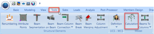
The recalculation of the mathematical model is made by selecting the corresponding command.
14. Select between 2D and 3D surface elements
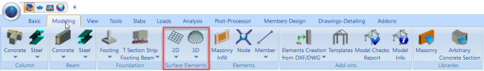
SCADA Pro offers the possibility to use surface elements to simulate areas of any shape and direction. Depending on the case you can use the 2D or the 3D surface elements.
The choice depends on the connection needs the surfaces together. In detail:
– In the case of an individual surface, ex. a raft or a slab, the you can choose either 2D or 3D.
– Όταν όμως υπάρχουν περισσότερες από μία επιφάνειες με κοινούς μεταξύ τους κόμβους, τότε χρησιμοποιείτε μόνο τα 3D πεπερασμένα στοιχεία προκειμένου οι κοινοί κόμβοι να δεσμευτούν αυτόματα. But when there are more than one areas with common nodes between them, then use only the 3D finite elements in order to commit automatically the common nodes.
Therefore, using 2D surface elements is limited, in contrast to 3D that can be used without restrictions.
But, Attention!
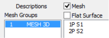 When using the 3D surface, all the related Mesh should belong to the same Mesh Group, for the purpose of achieving the automatic commitment.
Δημιουργήστε ένα πλέγμα και με την εντολή Εξωτερικό Όριο, ορίστε τις Επιφάνειες που ανήκουν σε αυτό, τροποποιώντας ενδεχομένως τα χαρακτηριστικά της κάθε μίας επιφάνειας,
Create a Mesh and using External Boundary command, set the surfaces belonging to it. If necessary, change the characteristics of each surface,
– either when creating:
 –or after, enabling Mesh and selecting the corresponding grid from the list.
In this way you can modify the characteristics of the selected surface (type, geometry, material) and  to update.
15. Model Checks – Errors and Warnings
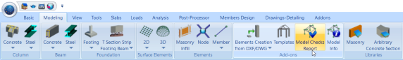
After creating the physical and then the mathematical model of the project, selecting “Model Checks“, the program checks the model for possible errors and warnings. Displays a .txt file with possible error messages relating to the physical or mathematical model (“Err”, number, level, message). Consult the messages and, where necessary, make the necessary modifications, using the corresponding commands.
“Err” is not always an error indication, it could be just a warning. The designer must correct the mistakes and take account of the warnings.
EXAMPLES
- The Beam 15 (2) is not connected at the end physically but is connected mathematically
concerns “Beam on Beam” condition, and this is a warning that requires no change. Close the window and continue.
- The Member (Colum) 10 at the end (0) is not connected
concerns column that in foundation level is not connected via horizontal linear member (strip footings, connecting beam) with another column.
Could be an error or just a warning, in cases of raft or independent footings, requiring no change.
- The Member (Beam) 5 at the end (1) is not connected
concerns beam that at its end is not connected to a column or to other beam. Could be an error or just a warning in case of beams defined as architectural protrusions.
16. What is the density of the surface finite elements
The “density” has to do with the regularity of the floor plan. Generally, as squared is a plan view, the lower density necessary (starting at about 0.10 – 0.15, otherwise 0.20 – 0.25).
17. How to model a slab of random shape
In many cases, the slabs of the model have not a rectangular shape thus requiring Modeling.
Start following the same procedure as for the rectangular slabs, meaning identification using one of the available modes.
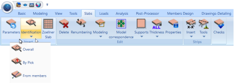
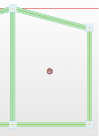
Slab is recognized but appears with a “?” next to the number, which means that needs modeling.
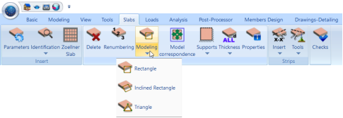
Click on Modeling and select Rectangle, then left click in the slab (somewhere inside its area).
Set successively the first and the second peak of the equivalent parallelogram (the two edges of the one diagonal).
 Then select
  and left click in the slab. Appears the Equivalent Rectangle.
Click on a side and appears the “x ” symbol on it.
Select then the physical members to assign to this side of the rectangle. These physical members acquire a dot in the middle having the same color as the side of the rectangle.
Complete matching on one side by pressing the right mouse button and continue the process for the other sides of the rectangle.
NOTE: Generally the program match automatically the members to the equivalent rectangular. This shown by the colored dots present.
Therefore, the above procedure should be followed only for members without colored dot.
Finally, assign each vertex of the equivalent rectangle (which is symbolized by a triangle) to the points of the physical model, making the reduction of the side length of the mathematical according the physical members.
18. How to simulate a slab with surface finite elements
The easiest way to simulate a slab with surface finite elements is through automatic conversion of a simple slab.
Through the field of Slab insert the slab as usual.
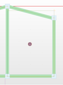
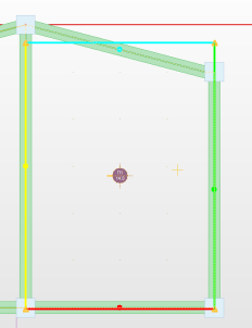
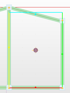
Start with setting free the nodes of the perimeter that belong to this slab, since they probably belong to a diaphragm.
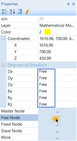
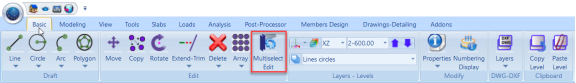
 This can be done for each node separately with reference to its data, by clicking the button next to “Free Node“. It can also be done for more nodes in group by using Ribbon “Basic>>Edit>>Multiselect Edit”.
Select the command “Properties” ![]() and left click in the slab:
and left click in the slab:
“Convert to Mesh” and then click “ΟΚ”.
![]()
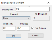
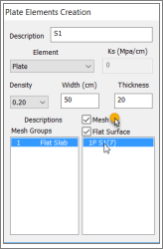
In the next dialog box, define the following parameters:
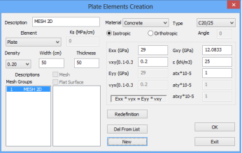
– Description, Element, Thickness equal to the thickness of the slab
– Density that depends on the form of the slab (usually a value around 0.20 is sufficient).
Also, if it is necessary, change the type of the concrete. Select “New” and then “OK”.
The program creates the mesh of the surface finite elements.
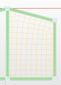
Then you need to calculate the model.
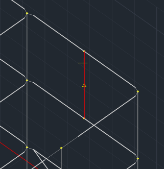
Last step is the segmentation of all peripheral beams, because of the nodes of the surface finite elements that were created, by using the command “Tools > Members> Beam-Plate Connection” ![]() .
.
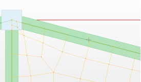
- By zooming on a beam, you see that in the mathematical model, it is broken in collinear members joined with the surface elements.
19. How to simulate the basement walls (3 ways)
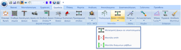
Simulation of the basement walls in SCADA can be in 3 ways:
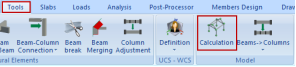
- Beams to Columns Conversion
- Smith Model
Γ. Diagonals Model
Α Way :
To simulate basement walls (level 0) by using the “Beams to Columns Conversion” do the following:
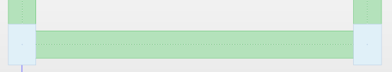
– Insert a beam in the position of the wall, having the same thickness with the wall, on level 1.
– Select the command “Beams to Columns Conversion” and in the dialog box that is displayed activate the “No. Of Columns” or “Max Column Length”, and type the corresponding number, “OK”.
NOTE: Consider to create columns having width of approximately one meter
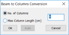
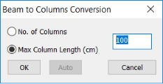
– Left click on the beam. It will be converted automatically and it will break into as many parts as the “No. of columns” or “Max column length” you have set.
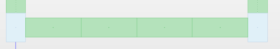
– Repeat the same procedure in the foundation level or select all the broken parts of level 1 and using the command Copy, copy them on level 0 at the corresponding position
– Select the mathematical model “Calculation”, to create unconnected nodes.
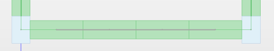
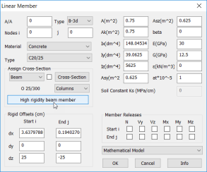
– Connect the nodes with linear members with high rigidity, similar to the walls, and ε=0.
Set the properties of the member, and then, just select the first node and all the others by window. The program will locate members from node to node.
In foundation you can place:
– either footings under each wall
and then connect them with high rigidity members,
– or footing beams.
To succeed this, because the walls are in contact (there is no min vacuum 10cm.), you should first, disable AutoTrim (from Display> Switches) and place the F/B without rigid parts (r. Offsets), clicking from node to node, or using the window selection. Finally, calculate the Mathematical Model to create the members of the footing beams, that will connect the nodes of the columns.
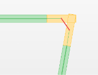
Β Way :
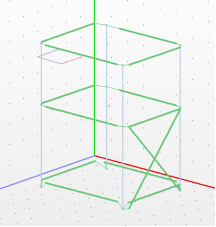
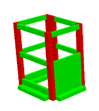
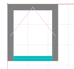
According to this method, the wall is modeled with two linear members placed in “X” order.
To implement “Model Smith” simulation:
- Level 1: in the position of the wall put a beam with the same thickness
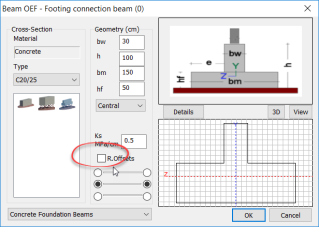
- Level 0: put the Strip Footing Beams or Footing Connection Beam
- Select ”Smith Model”
- Left click on the beam that is going to change automatically.
- The program inserts two linear members in “X” order between two columns and the parameters A, Ak, Asy, asz, and Iz of the members, on the border of the simulated wall, are changed automatically.

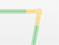
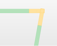
C Way :
Follow the “Smith Model” procedure.
Based on the “Diagonals” method, the basement wall is modeled with two linear members placed in “X” order (diagonal order).
NOTES:
- The main difference between the Smith Method and the Diagonals is that the second method simulates the wall, without changing the inertial characteristics of the members on the border, unlike the Smith method.
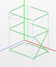
- The basic precondition for using these two methods for simulating walls is the presence of the mathematical model and the presence of the beams that will be transformed in X linear members. These beams must have the same thickness as the simulated walls.
Automatically the program calculates the rigid offsets of the members.
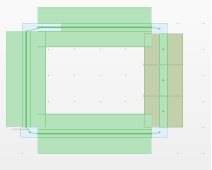
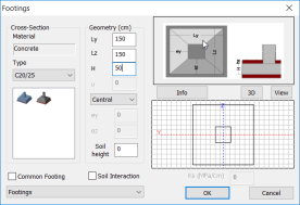
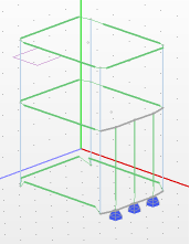
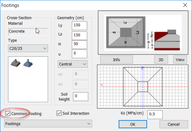
20. How to insert a common footing under 2 or more columns
Set all the parameters of the geometry of the footing to the corresponding window, enable “Common Footings” and then select successively the columns in which will be placed.
21. How to make individual changes in existing physical or mathematical elements
The renewed interface of SCADA Pro offers possibilities of making changes to the model, fast and easy, following the changes directly to your screen.
For individual changes you can select un element, either graphically, or through the “tree list” on the left, so that on the right appear its properties.
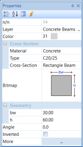
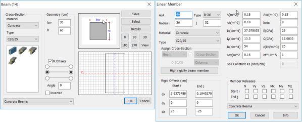
Physical section properties (beam)
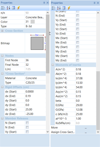 Mathematical member properties (beam)
Fields of properties displayed can be modified,
or by directly entering values,
![]()
or activating and deactivating the checkbox,
or by changing the selection,
either by selecting the command “More” for more modifications.
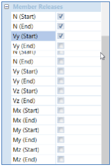
22. How to make total changes in existing physical or mathematical elements
To make changes in more elements simultaneously (all beams on all nodes of the raft, etc.) use the command “Πολλαπλές επιλογές”.
First select the command:

then all the elements for modifying , using the selection commands ![]() and right click to open the dialog box:
and right click to open the dialog box:
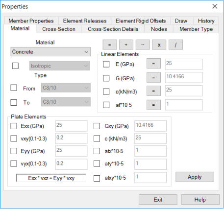
Inside this window you can find all the individual properties by category, and modify. Detailed description can be found in the relevant section of the manual.
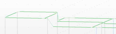
23. How to simulate a complex column section
SCADA Pro contains a large library of sections that covers the majority of cases. However, in some cases it is proposed the use of composite sections to simulate the model.
NOTES:
The most common cases where complex cross-sections are required:
–cases of parametric cross-sections, different from T-shaped and C sections, because not dimensioned by the program
–when only one section is not sufficient to give the fact properly
–when you need to insert a beam in the core ends
–when you want to set slabs and there are no beams
Simulation of composite sections, by composing rectangular cross section and joining them by high rigidity members.
Enter the physical sections, calculate the mathematical model and join the nodes by using high rigidity members.
24. Core simulation with columns and beam
Create the core using rectangular column sections and high rigidity members.
Define the beam that connects the ends of the wall core and complete calculating the mathematical model.
25. Differences between elements defined by physical cross sections and the corresponding members with section assignment
For SCADA Pro a static element consisting of the physical (cross section, surface) and the mathematical (members, nodes) model.
For making the model, the user can either:
– Set the physical section and then the mathematical member
– Set the mathematical member and assign the physical section
– Or both
The choice of how to build the model depends from case to case. For example:
- If you choose a dwg to start, then insert sections and simultaneously you can calculate also the mathematical model.
- If you select a template, then automatically entered members with section assignment.
- If you do not choose to use auxiliary, then start by introducing sections, creating levels and then the calculation of the mathematical model. At this point you can add members from node to node, with and without cross–section assignment.
NOTES:
– The existence of the mathematical model allows the 3D visualization and photorealistic
– Mathematics members may be with or without section assignment
– An item that is created by physical sections, obeys to “Structural Elements” tools, while
an item that is created by members, obeys to “Members” tools
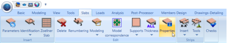
26. How to model a zoellner slab
y using ![]() command you can model a Zoellner slab.
command you can model a Zoellner slab.
Prerequisite for the Zoellner slab is, the insertion and the modeling of the normal slab first.
How to use the command:
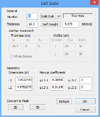
Select the command and the slab, clicking inside. Opens the dialog box:
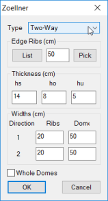
In “Type” επιλέγετε εάν η πλάκα με κενά θα είναι μίας ή δύο Διευθύνσεων (αμφιέρειστη ή τετραέρειστη).
In the drop-down list “Type”, select if the slab is connected in one or two directions.
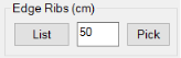 Then define solid zones’ widths (cm). Type the number and click the button “Pick”
 ![]() . Left click on the side of the beam considered as an outline of the slab. Then, the boundary of the solid zone will be placed in parallel with the beam at a distance equal to the width that was defined previously. The line is drawn (boundary of the solid zone) and with left click the direction is indicated.
. Left click on the side of the beam considered as an outline of the slab. Then, the boundary of the solid zone will be placed in parallel with the beam at a distance equal to the width that was defined previously. The line is drawn (boundary of the solid zone) and with left click the direction is indicated.
NOTES
The solid zones should be defined in a row and circularly, clockwise or counterclockwise.
If you press right click during the definition of the solid zone, the “Zoellner” dialog box opens, so that you can define different widths for the next solid zone.
After defining the latest solid zone, right click to open the window and complete it by typing thickness, ribs and domes widths.
In the next section the thickness of the slab is defined.
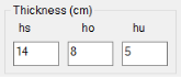 In “hs” type the slab’s total thickness (cm).
In “ho” type the up side solid slab’s thickness (cm).
In “hu” type the down side solid slab’s thickness (cm) for Sandwich slabs. Otherwise type 0.
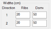
In Widths:
 Define ribs and domes widths:
Type the widths in each direction.
- Direction 1 is the direction parallel to the slab’s side that you will define when the program will ask you to do so. For Zoellner slabs on one direction, Direction 1 is the main slab’s direction.
- Direction 2 is the other one (vertical).
Activate the checkbox Activate the checkbox ![]() to receive only whole domes.
to receive only whole domes.
Click “OK” to display the mathematical model of the selected slab. Then the program asks you to define Direction 1 (the side of the slab, which will be parallel to the beam of the first direction).
 Select the side of the slab’s model and the gap with the defined geometry is placed automatically in the center.
 To define where to start putting the domes, first click on a dome’s vertex and then on a slab’S vertex.
Automatically the solid slab is converted to a Zoellner slab:
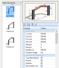
27. How to add a template over another template or existing model
The access to the Templates tool can be in 2 ways:
1st way:
– – Left-click on one of the icons of the start screen, select the type of template.
Concrete / Steel
Surface
Masonry / Timber
– Give a name to your file and automatically opens the dialog box of the templates.
2nd way:

– Select MODELING>ADD-ONS>TEMPLATES and
– automatically opens the dialog box of the templates.
NOTES:
If the file already contains elements, select the insertion point on the desktop to open the templates window.
If you want to superimpose a template on an existing structure, then
– Open the 3D view of the existing structure
– Select “Templates” command,
– By left-click select the node, that will be the insert point of the new construction, activating the proper snap (example: end point), and considering that this point will be identified with the origin of the template.
– Set the parameters of new construction, ensuring to have the same openings in width with the existing structure.
– Press ΟΚ and the template inserted over the existing.
28. How to convert lines of an auxiliary file in SCADA lines
By inserting an auxiliary file (dxf-dwg) in SCADA’s environment, there is the opportunity to use the lines of the drawing file only as snap points. An additional feature that gives you SCADA is to convert the lines of the drawing file on lines of SCADA. So, you can operate the auxiliary file as a design entity of SCADA without need of redesigning. The procedure is:
– Import the auxiliary file
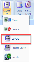
– Select the command Basic->DWG-DXF->Layers
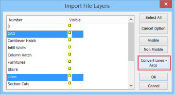
– In the dialog box displays the list of all the layers of the auxiliary file. Select one or more layers, using the left mouse button and Crtl, and the command “Convert Lines, Arcs”. Lines and arcs belonging to selected layers will be converted to design elements of SCADA.
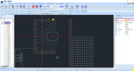
– Selecting a line of the selected layer, the properties display as part of SCADA that now belongs to Layer “Lines-Cycles”.
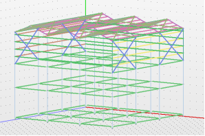
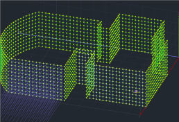
29. How to use an auxiliary file to create a finite surface elements model
For modeling structures of finite surface elements with complex floor plans, SCADA Pro provides an intelligent way, using a design and the templates tool, allows you to “build” your model easily and quickly.
The procedure includes the design insertion and the lines conversion.
 Analytically:
1. Import a .dxf or .dwg file
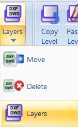
2. Select DWG – Layers command
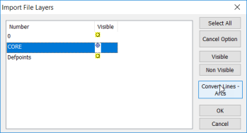
3. Select from the list the layer of the outline and press “Convert Lines button, Arcs“.
NOTES
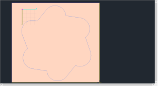
 – If you don’t have any .dxf or.dwg file, you can you can draw the contour line in the XZ level of the desktop using the Draft commands.
–The dwg file that you use as an auxiliary file is inserted in the SCADA environment in active XZ level identifying the origin to the upper left point of the project ![]() .
.
– Lines and / or polylines defining the outline, in order to be recognized as SCADA lines, should belong to a separate layer, and using ” Convert Lines, Arcs” to obtain the recognition.
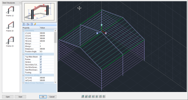
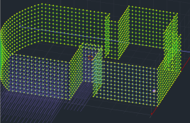
4. In “Modeling” select “Surface elements – 3D”>>“Front View Identification”, and using ![]() , select all the floor plan
, select all the floor plan
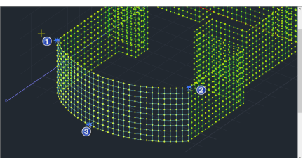
5. Right click and opens the Templates window:
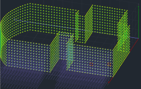
The program automatically recognizes the outline mesh. Proposes by default a height and creates facets on the global axes.
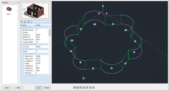
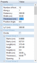
The user must define the number of floors and the individual altitudes, the thickness of the walls and openings on each view.
After you complete the process for each view and each opening, insert the body on the desktop by clicking the OK button.
Loads
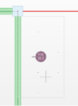
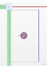
30. How to insert a Linear Load on a cantilever (or slab)
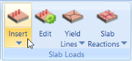
Select:
– Insert – Slab Loads > By Pick
– Load Type > Linear and type the value (KN/m)
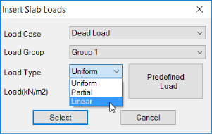
– Click Select and select also the slab. Define graphically the line for the load application.
31. How the Load distribution on the surface works
![]()
The new version of Scada Pro includes a new tool for the automatic distribution and application of the loads on the mesh area.
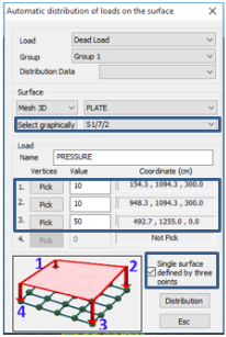
Select the command, and on the dialog box that opens, define:
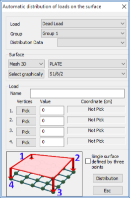
– The type of load from the “Load” field and the group from the “Group” field.
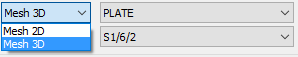
– In the “Surface” field, select the type of the surface and the surface group that you wish to load.
![]()
NOTES
 In case that the selected mesh group has more than one surfaces you must select from the list, the preferred surface as well.
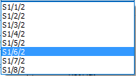
The load application can be performed graphically as well by clicking the button ![]() .
.
The dialog box closes automatically so that you can identify the surface by clicking on one of its shell element.
Then the dialog box reopens with the pointed out surface identified.
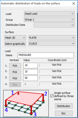
On the “Load” field give a name for the load. Afterwards, define the way of the load distribution on the selected surface.
The definition can be performed graphically:
- By pointing the 4 corners of the surface and setting the load value.
- By pointing 3 points the first two of which define a straight line that the first load value will be applied, and the third which defines the height that the second load value will be applied.
It isn’t necessary for these points to belong one the same level, while the outline of the surface can contain lines and arcs.
More specifically:
- On flat surfaces:
Point the 4 corners that define the surface by clicking successively the buttons ![]() for each corner as shown in the image below.
for each corner as shown in the image below.
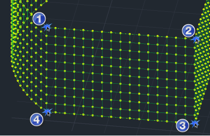
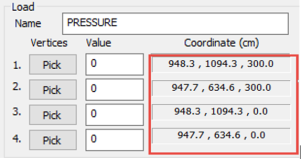
In this way, the coordinates for the 4 corners are automatically recognized and filled in.
Next you set the pressure values (in kN/m2) for each corner point
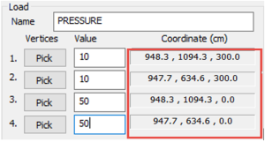
Finally, click the buttons ![]() and
and ![]() .
.
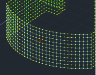
The load distribution on the selected surface is completed and is graphically represented on the elements of the current surface.
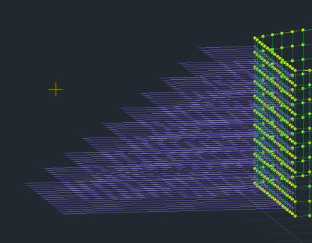
- On consecutive surfaces:
Now you are able to distribute automatically the loads on consecutive areas.
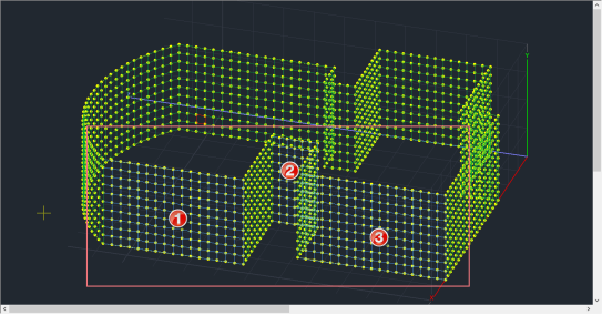
A similar process is followed with the below differences being the only ones:
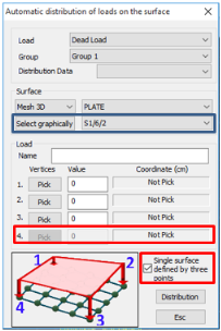
- Using the “Select graphically” command you only select one element form one of the surfaces that are to be loaded.
- Check the command “Single surface defined by three points” and the 4th option is automatically disabled.
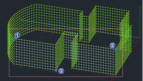
As previously described, using the ![]() button, you point to the 3 points that define the combined area.
button, you point to the 3 points that define the combined area.

Finally, click the buttons ![]() and
and ![]() .
.
- The load distribution on the selected surface is completed and is graphically represented on the elements of the current combined surface.
![]()
![]()
- In order to distribute the loads to the rest of the surfaces, select again the command
 and at the dialog box, click
  and select an element from the next surface that is automatically recognized and selected from the list
  . Click the buttons
  and
and  .
.
- Follow the same procedure for the third surface.
- On curved surfaces:
Follow the same procedure:
Graphical selection with one click.
Check the option “Single surface defined by three points” and the 4th option is automatically disabled. Define the surface by pointing to the three points that define the surface using the ![]() buttons. Fill in the pressure values (in kN/m2) and click
buttons. Fill in the pressure values (in kN/m2) and click ![]() and
and ![]() .
.
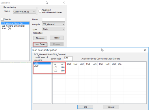
32. What is the meaning of LG, the deference from LC and how to use them
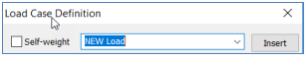
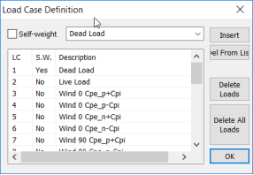
“Loads” field commands allow to define Loads and respective Groups, where all the project loads are included.
LC = Load Case: Dead , Live , Snow ecc.
Defining them is necessary, because is the basic requirement for the importation of the construction loads. Each load belongs to one of these (Load Cases).
By default, the program has predefined two Load Cases:
- Dead Loads (L.C.=1)
- Live Loads (L.C.=2)
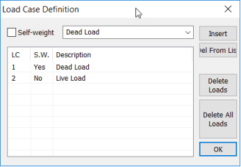
S.W. column, indicates the involvement of the same weight on that load.
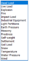
Apart from the default, Dead and Live, can be introduced other loads, either by selecting from the list, or by typing in the list and then “Insert”.
LG = Load Group: are subgroups of the LC. They serve to have a better overview of the loads of the structure, especially in the 3D display (especially if we choose a different color for each LG).
Load Groups creation is an optional procedure. For each load there is by default one group “Group1”.
NOTES
In case you define additional Groups for each load,
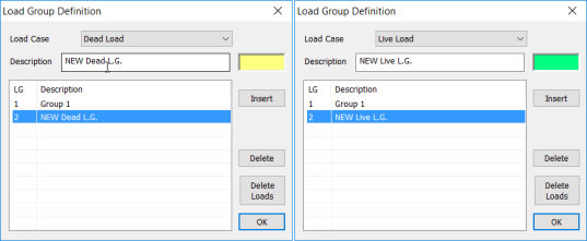
you should note that:
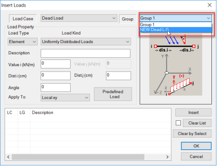
– When inserting the loads, you must select the corresponding Group.
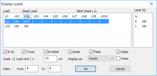
– In Loads display, Groups shown separately
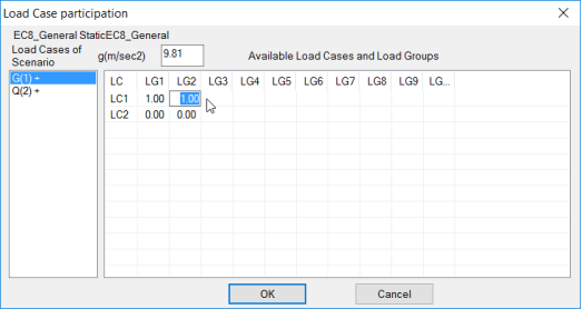
– In Loads participation for the Analysis Scenario, the unit “1” should be set manually in the additional LG to take into account in the analysis.
Analysis
33. How to create load combinations for seismic analysis scenarios
After the execution of a seismic analysis scenario, the combinations automatically generated by the program. Selecting the command “Combinations” opens the table with the combinations of the active seismic scenario.
The same results are derived from the “Default Combination” button, which completes the table with the combinations of the active scenario analysis. ![]()
The default combinations of the executed analysis, are automatically saved by the program.
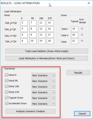
34. How to add the combinations of Wind and Snow loads together with the seismic combinations, using the automation "Wind -Snow"
SCADA Pro provides an automated way to combine together, Wind, Snow and seismic loads.
NOTE
This automation requires, the automatic procedure for the calculation and distribution of wind and snow loads, and the automatic creation of loads and scenarios.
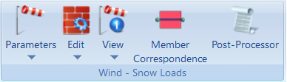
Keeping the above requirements, it is possible to create wind and snow combinations automatically using the command ![]() .
.
-Run the earthquake scenario and all the static scenarios of wind and snow
–Activating the earthquake scenario and select the command “Combinations” and “ Default Combination “.
Automatically filled combinations of active seismic scenario.
– For the automatic creation and other combinations (wind and snow) press ![]() .
.
Automatically filled in the coefficients of wind and snow scenarios, providing a complete file of combinations of all the loads.
Press ![]() to save it for using in Members Design.
to save it for using in Members Design.
35. How to enter an additional load and combinations in analysis
Besides the “ Default Combination” you can add more with loads of other scenarios, following the manual way:
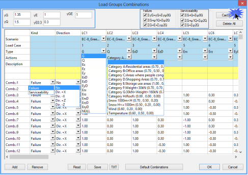
– First type in the partial safety factors γG, γQ, γE, and check the Failure and Serviceability equations that you want to be considered.
– Then fill in the “LC” columns:
– Select the previously created Scenario from the scenarios list.
– Select the Load Type between Dead, Live, Seismic, or Null. Null is selected for other type of loads like Wind, Temperature, etc.
– In the Actions line select the corresponding action from the list.
– In the Description line, you can type in a description. This is optional.
– Do the same for all Load Cases and then click![]() . Combinations’ lines are filled in with the appropriate coefficients automatically.
. Combinations’ lines are filled in with the appropriate coefficients automatically.
–  “Type” column indicates which type of limit state is examined through the defined combination
 ![]() .
.
– “Direction” column indicates in which direction the capacity of the structure will be examined during the Capacity Design procedure for the specific combination.
– ![]() buttons allow to add or remove lines and columns since they have been selected, like in an excel file.
buttons allow to add or remove lines and columns since they have been selected, like in an excel file.
– You always have to ![]() the combination as a CMB file in the project’s folder. You will need this file during “Post-Processor” and “Members Design”.
the combination as a CMB file in the project’s folder. You will need this file during “Post-Processor” and “Members Design”.
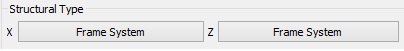
36. How to calculate the Behavior factor “q” automatically by the program and how you determine the "Structural Type "
The “Behavior factor q” of the structure results from a computation procedure. Additionally, the “Structure type” follows certain criteria. SCADA Pro yields both of them automatically.
Complete all the parameters fields
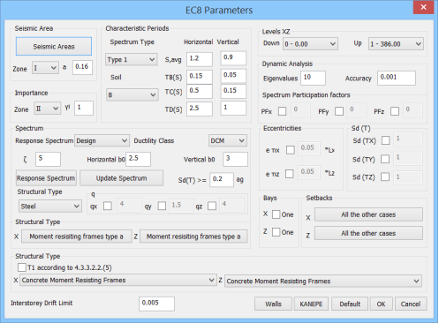
leaving the following boxes blank:
![]()
as well as the following options
without any changes.
Choose “Ok” and using the “Automatic procedure” run an initial analysis.
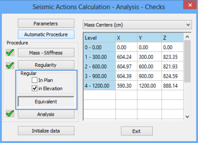
Click “Exit” to close the dialog box and choose the “Checks” command ![]() of the “Results” menu at the ribbon, to open the “Seismic analysis control coefficients” dialog box.
of the “Results” menu at the ribbon, to open the “Seismic analysis control coefficients” dialog box.
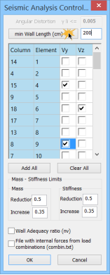 There, you are asked to assign a value to the minimum length that a vertical member must have in order to be regarded as a wall instead of a column. Click the
 ![]() button, and automatically, all the walls are checked in each direction.
button, and automatically, all the walls are checked in each direction.
As far as the “Wall adequacy” is concerned, the relevant .txt file contains the computation of the shear acting to each wall, at each level of the structure and for all the load combinations considered.
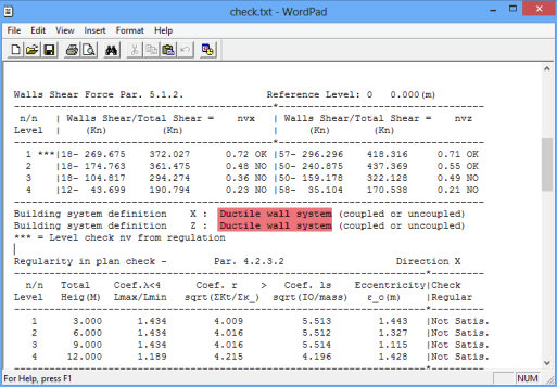
Since the “Building system definition” has been determined, it should be included in the “Parameters” dialog box. With these changes, conduct the analysis for a second time. Now, the proposed values for the “Behavior coefficient q” can be found in the “Parameters” dialog box. For the example considered, in the “q” area, one can read:
![]()
The proposed values may be kept or altered (the latter one is an option that could be utilized from the beginning of the procedure, however, in this occasion the software would not propose any values, at all).
![]()
Click “Ok” and conduct the analysis one more time, in order for the q values to be accounted for.
37. Prerequisites for the execution of a push over analysis
Important prerequisite for the implementation of the nonlinear analysis scenario is the existence of the steel reinforcement, which is calculated only when the cross-sections are designed according to Eurocode 2 considering the modified strength value of the materials.
- Initially preceded the modeling of the structure with new materials (NOT allowed qualities the old qualities of materials (B and STI)), which will be adjusted based on individual strength and safety factors.
- Then it should be a first analysis, using scenario Eurocode 8 (static or dynamic).
- The reinforcement results from design ONLY according to Eurocode 2 considering the modified strength value of the materials.
- As the materials of the existing structure are considered the modern materials with modified properties with respect to the corresponding safety factors. The materials of the existing structure are not type of Β and STI (old type of materials). If the structure studied has materials of type B and STI, then for the definition of the materials in the design parameters field and before the preliminary design, use the properties of the modern materials modified with the safety factors according to EC8 part3.
- Since the preliminary design has been completed and the existing steel reinforcement had been inserted in the structural model and before the creation of the pushover analysis scenario, it is demanding to precede the “Strength calculation (Pushover)” by selecting the corresponding command.
38. How to model Masonry Infill
Using this command you can model the masonry infills. Modelling is made with two diagonal bars at zero weight (wall loads have already considered as linear loads on the beam members). Select the command and left click on the upper beam member of the panel that contains the masonry infill.
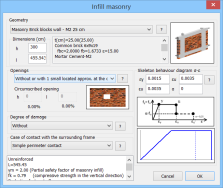
Opens the dialog box with the relative parameters
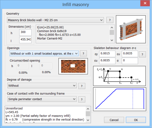
In “Geometry”, select from the drop-down list the wall after created in the library of masonry, otherwise press![]() to open the library of mansory and define it.
to open the library of mansory and define it.
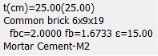
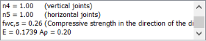
Displaying the wall properties as the total thickness t (mantle and wall), the type of masonry with its strength and the type of the corresponding mortar strength.
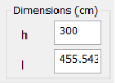
In “Dimensions” the editable height (h) and width (l) properties of the panel as calculated by the program are displayed.
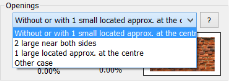
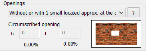 “Openings” concerning the wall openings. Select from the list one of the options.
NOTE
Choosing “Other case” you must type the corresponding dimensions.
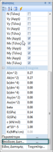
 Define the Openings in order to calculate the reduction factor of the compressive strength n1.
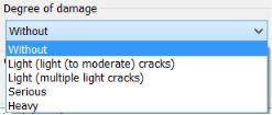
Define the Degree of damage in order to calculate the reduction factor of the compressive strength rR.
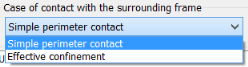
At the end, select the Case of contact with the surrounding frame, affecting the calculation of the reduction factor n3 per slenderness.
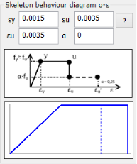
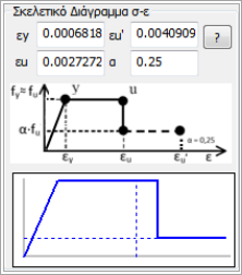
Skeleton behaviour diagram tension – deformation for the masonry infill.
The graph is drawn automatically.
For unreinforced masonry you have to type the corresponding values. For reinforced masonry, εy and εu are calculated automatically. In both cases the values can be modified by the user.
α factor is the proportion of the residual strength after fracture and conserns only the reinforced masonry, such as the reduced distortion total failure ε’u.
The results of the choises can be overseen here:
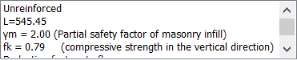
the compressive strength, the elastic modulus, the partial safety factor, etc.
Press ΟΚ to create automatically the two diagonal members in the panel.
The masonry infills can be inserted either in the plan view of each storey or in 3D View.
Reporting, editing and modification can be performed through the “Assign Cross-Section” command of the properties.
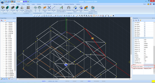
Left click on a diagonal member and in Properties select “Assign Cross-Section” to open the respective dialog box and make the changes.
ATTENTION
Changes concern only the selected member. To change other members you must do the same procedure for each one.
ATTENTION
Changes inside the library of the masonry infill are not mirrored to the existing masonry members. In order to update the properties of the members of the masonry infills to reflect the new data, corresponding to the updated library, you must open the “Plate Elements Creation” form, select it and click ![]() .
.
In elastic analysis may be considered a cross device (hence one diagonal is compressed and the other is stretched, while no need iterations in each solution to be kept in the model only compression diagonals), giving each diagonal half of stiffness.
In inelastic analysis can be used (since is available the appropriate software) a pair of cross diagonals with stiffness ΕΑρ each, but unilateral statute law (only in compression mode). If the filling walls have openings, the respective statute law modified appropriately, so as to approach the adverse overall influence of the openings.
39. Πώς προσομοιώνονται οι τοιχοπληρώσεις
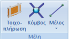 Η ομάδα εντολών “Μέλη” περιλαμβάνει τις εντολές για τον καθορισμό και την εισαγωγή των Τοιχοπληρώσεων.
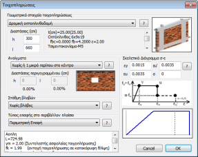
Με την εντολή αυτή μπορείτε να εισάγετε τις τοιχοπληρώσεις της κατασκευής σας σύμφωνα με τα όσα προβλέπει ο ΚΑΝ.ΕΠΕ.
Η προσομοίωση γίνεται με δύο διαγώνιες ράβδους με μηδενικό ειδικό βάρος (αφού τα φορτία των τοιχοπληρώσεων έχουν δοθεί σαν γραμμικά φορτία πάνω στα μέλη των δοκών) και με επιφάνεια διαστάσεων σύμφωνα με τα όσα προβλέπει ο ΚΑΝ.ΕΠΕ.
Αφού επιλέξετε την εντολή, δείχνετε με το ποντίκι το μαθηματικό μέλος της άνω δοκού του φατνώματος που θα τοποθετηθεί η τοιχοπλήρωση.
Στη συνέχεια εμφανίζεται το παρακάτω πλαίσιο διαλόγου
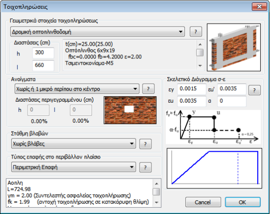
Στην ενότητα “Γεωμετρικά στοιχεία τοιχοπλήρωσης”, από τη λίστα επιλέγετε την τοιχοπλήρωση που έχετε προηγουμένως δημιουργήσει στην βιβλιοθήκη της τοιχοποιίας. Στο παραπάνω παράδειγμα έχει επιλεγεί η δρομική οπτοπλινθοδομή. Πιέζοντας το σύμβολο ![]() εμφανίζεται το πλαίσιο διαλόγου της βιβλιοθήκης της τοιχοποιίας, όπου έχετε τη δυνατότητα να δημιουργήσετε και να τροποποιήσετε τις τοιχποπληρώσεις. Στο εικονίδιο δεξιά εμφανίζεται ο αντίστοιχος τύπος της τοιχοπλήρωσης.
εμφανίζεται το πλαίσιο διαλόγου της βιβλιοθήκης της τοιχοποιίας, όπου έχετε τη δυνατότητα να δημιουργήσετε και να τροποποιήσετε τις τοιχποπληρώσεις. Στο εικονίδιο δεξιά εμφανίζεται ο αντίστοιχος τύπος της τοιχοπλήρωσης.
Στο επόμενο πεδίο:
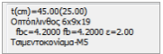
Εμφανίζονται οι ιδιότητες της τοιχοπλήρωσης, όπως το πάχος t (συνολικά με τον μανδύα και το καθαρό), το είδος του λιθοσώματος με την αντοχή του, καθώς και το είδος του κονιάματος με την αντίστοιχη αντοχή του.
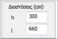 Στην επόμενη ενότητα εμφανίζονται αυτόματα το ύψος (h) και πλάτος (l) του φατνώματος όπως υπολογίστηκαν από το πρόγραμμα με δυνατότητα επεξεργασίας.
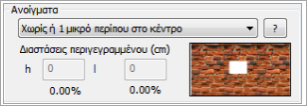 Η επόμενη ενότητα αφορά στον ορισμό των ανοιγμάτων της τοιχοπλήρωσης. Επιλέγετε από τη λίστα μία από τις επιλογές.
ΣΗΜΕΙΩΣΗ
Εάν επιλέξετε “Άλλο” πρέπει να ορίσετε τις διαστάσεις του περιγεγραμμένου στα ανοίγματα ορθογωνίου.
Η επιλογή των ανοιγματων γίνεται προκειμένου να υπολογιστεί ο μειωτικός συντελεστής της θλιπτικής αντοχής n1.
Πιέζοντας το πλήκτρο ![]() εμφανίζεται επεξηγηματικό κείμενο με την αντίστοιχη παράγραφο του ΚΑΝ.ΕΠΕ.
εμφανίζεται επεξηγηματικό κείμενο με την αντίστοιχη παράγραφο του ΚΑΝ.ΕΠΕ.
![]() Η επόμενη ενότητα αφορά στις βλάβες της τοιχοπλήρωσης από όπου επιλέγετε και την αντίστοιχη στάθμη για να υπολογιστεί ο μειωτικός συντελεστής rR.
Η επόμενη ενότητα αφορά στις βλάβες της τοιχοπλήρωσης από όπου επιλέγετε και την αντίστοιχη στάθμη για να υπολογιστεί ο μειωτικός συντελεστής rR.
Πιέζοντας το πλήκτρο ![]() εμφανίζεται επεξηγηματικό κείμενο με την αντίστοιχη παράγραφο του ΚΑΝ.ΕΠΕ.
εμφανίζεται επεξηγηματικό κείμενο με την αντίστοιχη παράγραφο του ΚΑΝ.ΕΠΕ.
![]()
Η επόμενη επιλογή αφορά στον τύπο επαφής της τοιχοπλήρωσης στο περιβάλλον πλαίσιο.
Η επιλογή του τύπου επηρεάζει τον υπολογισμό του μειωτικού συντελεστή n3 λόγω λυγηρότητας. Με το πλήκτρο ![]() εμφανίζεται το αντίστοιχο επεξηγηματικό κείμενο.
εμφανίζεται το αντίστοιχο επεξηγηματικό κείμενο.
 Η επόμενη ενότητα αφορά στη δημιουργία του σκελετικού διαγράμματος τάσεων – παραμορφώσεων της τοιχοπλήρωσης.
Εδώ και στα αντίστοιχα πεδία ορίζετε, για την άοπλη τοιχοποιία, την ανηγμένη παραμόρφωση διαρροής εyκαι την ανηγμένη παραμόρφωση οιονεί-αστοχίας εuσύμφωνα με τον ΚΑΝ.ΕΠΕ. Στο γράφημα σεχδιάζεται αυτόματα το σκελετικό διάγραμμα. Προκειμένου για οπλισμένη τοιχοποιία, οι τιμές εy και εuυπολογίζονται αυτόματα. Και στις δύο περιπτώσεις οι τιμές μπορούν να τροποποιηθούν προαιρετικά από το μελετητή. Ο συντελεστής α όπως φαίνεται και στο γράφημα είναι το ποσοστό της εναπομένουσας αντοχής μετά τη θραύση και αφορά μόνο την οπλισμένη τοιχοποιία όπως και η ανηγμένη παραμόρφωση πλήρους αστοχίαςε’u.
Τέλος η ενότητα
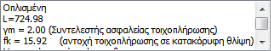
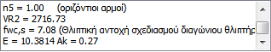
περιέχει, για τις παραμέτρους που αναφέρθηκαν παραπάνω, τα αποτελέσματα των επιλογών, καθώς και την τελική θλιπτική αντοχή σχεδιασμού του διαγώνιου θλιπτήρα, το αντίστοιχο μέτρο ελαστικότητας, την επιφάνεια Ak της διατομής των διαγώνιων ράβδων καθώς και το μήκος τους L.
Επιλέγοντας ΟΚ, δημιουργούνται αυτόματα οι δύο διαγώνιες ράβδοι στο φάτνωμα. Η εισαγωγή των τοιχοπληρώσεων μπορεί να γίνει είτε στην κάτοψη του κάθε ορόφου, είτε στο φορέα σε τρισδιάστατη απεικόνιση.
 Η εκ των υστέρων αναφορά, επεξεργασία και τροποποίηση των τοιχοπληρώσεων γίνεται μέσα από την ενότητα των ιδιοτήτων. Με την επιλογή μιας διαγώνιας ράβδου της τοιχοπλήρωσης επιλέγετε από τις ιδιότητες αριστερά την “Απόδοση Διατομής” και εμφανίζεται το πλάισιο διαλόγου
με τα αντίστοιχα στοιχεία της τοιχοπλήρωσης που έχετε ήδη εισάγει. Εδώ μπορέιτε να αλλλάξετε όποιο στοιχείο θέλετε.
ΠΡΟΣΟΧΉ
Δεν γίνεται αυτόματα ενημέρωση των τοιχοπληρώσεων της κατασκευής εάν αλλάξετε κάποιο δεδομένο στην τοιχοπλήρωση μέσα στη Βιβλιοθήκη της τοιχοποιίας. Για να γίνει η ενημέρωση, θα πρέπει να κάνετε αναφορά σε κάθε ράβδο των τοιχοπληρώσεων με τη διαδικασία που περιγράφηκε προηγουμένως, και να πατήσετε OK στο αντίστοιχο πλαίσιο διαλόγου.
ΠΑΡΑΤΗΡΗΣΕΙΣ
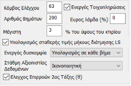
Δίνεται η επιλογή στον χρήστη αφότου έχει εισάγει τις τοιχοπληρώσεις να επιλέξει εάν θέλει ή όχι να τις λάβει συνολικά υπόψη στην Pushover ανάλυση μέσω της επιλογής“Ενεργές Τοιχοπληρώσεις” ![]() που βρίσκεται στο παράθυρο των Παραμέτρων του σεναρίου της.
που βρίσκεται στο παράθυρο των Παραμέτρων του σεναρίου της.
Στις ελαστικές αναλύσεις επιτρέπεται να θεωρούνται σε χιαστί διάταξη (άρα η μια διαγώνιος θλίβεται και η άλλη εφελκύεται, ενώ δεν προκύπτει ανάγκη διαδοχικών προσεγγίσεων σε κάθε επίλυση ώστε να κρατιούνται στο προσομοίωμα μόνο οι θλιβόμενες διαγώνιοι), δίνοντας σε κάθε διαγώνιο το ήμισυ της δυστένειας.
Στις ανελαστικές αναλύσεις μπορεί να χρησιμοποιείται (εφόσον διατίθεται το κατάλληλο λογισμικό) ζεύγος χιαστί διαγωνίων με δυστένεια ΕΑρ η καθεμιά, αλλά μονόπλευρο καταστατικό νόμο (λειτουργία μόνο σε θλίψη). Στην περίπτωση που οι τοιχοποιίες πλήρωσηςέχουν ανοίγματα, οι αντίστοιχοι καταστατικοί νόμοι τροποποιούνται κατάλληλα, ώστε να προσεγγίσουν τη δυσμενή εν γένει επιρροή των ανοιγμάτων.
Design
42. How to import the designs and the details of a dimensioned model in Drawing-Details environment
The program reads the geometry data from the Modeling and Dimensioning results from the relevant section.
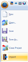
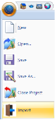
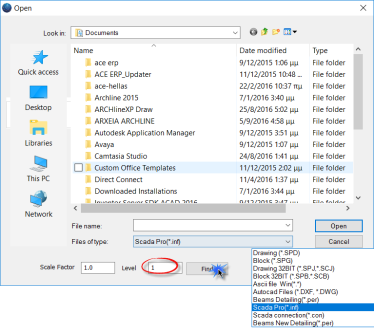
Selecting “Import” command opens the following dialog box for choosing the project’s folder.
Then select:
– the type of project from Files of Type
– the number of the floor
– the Scale factor
and press Find.
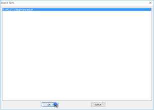
In the dialog select the path and press ΟΚ
Indicate the insertion point and insert the design of the selected level. Repeat for all levels
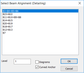
Respectively, choosing Beam Alignment (old and new) in the Find path, It takes you into a new window
Indicate the insertion point and insert the design of the selected level. Repeat for all levels
43. Where is the design of a surface with surface finite elements
For such surfaces, the reinforcement results Asx, Asz above and below, in cm2 / m, for each combination.
The favorable reinforcements resulting from the envelope of all combinations.
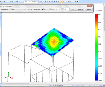
From reinforcements tables, engineer can convert the square centimeters per meter of width required, in reinforcement diameter (ex. F14 / 10).
44. How to modify reinforcements to a column already dimensioned
The New Column’s Editor – “Column’s Detailing” of SCADA Pro is part of an innovative new group of tools to manage the design details of the columns.
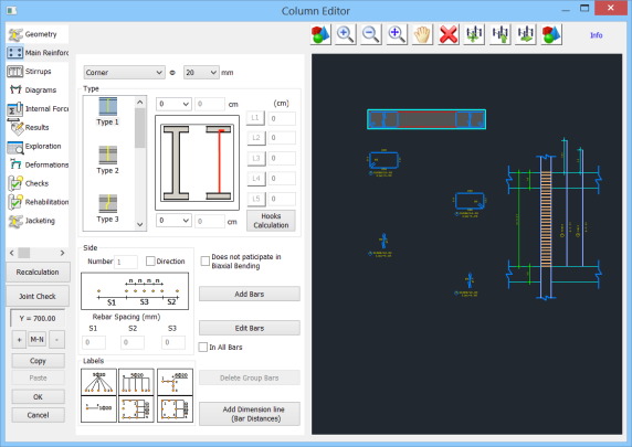
In the “Main Reinforcement” section you can modify the main steel reinforcement of the column.
Main reinforcement consists of two categories of bars with respect to their position inside cross-section; corner and side bars. Moving the mouse near the bar in the drawing, the ![]() state is activated, so you can read the characteristics (category, type).
state is activated, so you can read the characteristics (category, type).
The procedure to make a modification is first to select the command, then to show the rebar and then follow the edit process:
- To modify the diameter and type of corner bars
- To modify the number, diameter and type of lateral bars
- To insert lateral bars when there are not
- To delete bars
- To enter dimensional lines
- To exclude a bar out of control in Biaxial Bending
- To apply the modifications to all the same bars
The steps to be followed in any intervention on the bars and the stirrups and the respective checks, in accordance with these procedures, refer to the detailed manual entitled CHAPTER B “COLUMN’S DETAILING”
45. How to modify reinforcements to a beam already dimensioned
The New Column’s Editor – “Beam’s Detailing” of SCADA Pro is part of an innovative new group of tools to manage the design details of the beams.
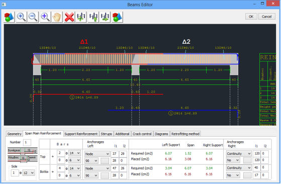
The “Span Main Reinforcement” unit consists of tools useful for the modification of the main steel reinforcement of the selected span.
The “Support Reinforcement” tab contains tools useful for the modification of the steel reinforcement of the supports of the selected beams.
The “Stirrups” tab contains useful tools for the modification or the addition of stirrups on spans and supports of the selected beam.
The “Additional” tab contains useful tools to modify or add additional rebar for shear or bending resistance, on spans and supports of the selected beam.
“Crack control” unit contains tools useful for the modification or addition of rebar against the concrete cracking, on spans and supports of the selected beam, on the top and bottom.
The steps to be followed in any intervention on the bars and the stirrups and the respective checks and diagrams, refer to the detailed manual entitled CHAPTER A “BEAM’S DETAILING”
46. How to apply the Capacity Design

The “Capacity Design” unit contains the commands to execute and display the capacity design results. Capacity Design is calculated per level. It should be made wherever necessary and always precedes the design of columns and walls.
For the performance and appearance of the capacity design results select the command Design:
Single
This command is used to apply capacity design on a single node. Select the command and left click on the node.
Overall
This command is used to apply capacity design on every node of the current level. Select the command and repeat for the other levels.
Notes:
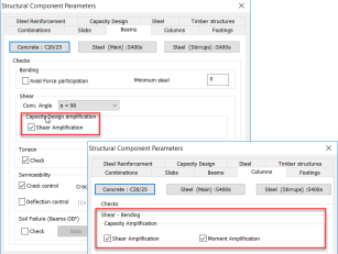
A prerequisite for the single and overall nodes capacity design, is preceded by the dimensioning of the beams, and to be selected “Capacity Amplification” in Beams and Columns fields in the Dimensioning Parameters window.
The Capacity Design should be done wherever required and always precedes the design of columns and walls.
The characterization of the nodes is a process which, if not performed by the user, the program will consider all nodes “free” in both directions.
In the section of parameters Dimensioning “Capacity Design”
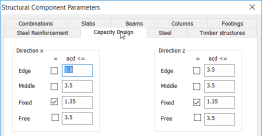
specify the x and z parameters to be used when the capacity control.
More specifically define the upper limit of the acd coefficient.
Generally, the value of acd defined must be less than or equal to the value of seismic behavior factor q.
For the anchoring positions of columns acd is taken equal to 1.35.
– Check the corresponding option and enter the value you want.
– If you do not check any option, the program will take into account the price of acd that will calculate.
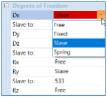
– Determining the type of node will be using “Node Releases“ command.